1: Direction fields.

Ordinary differential equations.

An ordinary differential equation (ODE) is an equation relating the derivatives of some unknown function \(y\) of a single variable \(x\). To solve the equation is to find the full family of functions satisfying the equation. Typically, there are infinitely many solutions to a given ODE if there is a solution at all.

The order of the ODE is highest order of derivative that appears in the equation. A typical first-order ODE can be expressed in the form

(1)\[y' = f(x,y).\]

A differential equation together with one or more initial values is called an initial-value problem (IVP). Typically, the number of initial values needed to obtain a unique solution is equal to the order of the differential equation. For example, the data

(2)\[\begin{split}y' &= y + \sin x,\\ y(0)&=-\frac{1}{2}\end{split}\]

define a first-order IVP with a unique solution. This course will primarily focus on the development of (approximate) numerical solutions to first-order IVPs.

Direction fields for first-order ODEs.

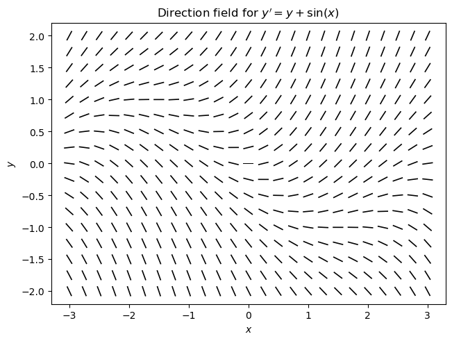
A direction field (or slope field) is a graphical visualization for an ODE consisting of short line segments which are tangent to the unique solution to the ODE that passes through the midpoint of the line segment. Given an ODE of the form (1) a direction field can be generated by evaluating \(f\) on a mesh of points in the \(xy\)-plane and sketching a line segment with slope \(f(x,y)\) at the mesh point \((x,y)\).

Creating direction fields with Python.

Below we generate a direction field with window \([-3, 3]\times [-2, 2]\) for the ODE (2). We use two popular Python packages for this task. The NumPy package provides efficient routines and data structures for scientific computing. MatPlotLib is a visualization library.

# import numpy and matplotlib.pyplot with conventional shorthands
import numpy as np
import sympy
from matplotlib import pyplot as plt

plt.style.use("dark_background")

# define ODE RHS
f = lambda x, y: y + np.sin(x)
# set window boundaries
xmin, xmax = -3, 3
ymin, ymax = -2, 2

# set step sizes defining the horizontal/vertical distances between mesh points
hx, hy = 0.25, 0.25

# sample x- and y-intervals at appropriate step sizes; explicitly creating array of doubles
xvals = np.arange(xmin, xmax + hx, hx, dtype=np.double)
yvals = np.arange(ymin, ymax + hy, hy, dtype=np.double)

# create rectangle mesh in xy-plane; data for each variable is stored in a separate rectangle array
X, Y = np.meshgrid(xvals, yvals)
dx = np.ones(X.shape)
# create a dx=1 at each point of the 2D mesh
dy = f(X, Y)
# sample dy =(dy/dx)*dx, where dx=1 at each point of the 2D mesh
# normalize each vector <dx, dy> so that it has "unit" length
[dx, dy] = [dx, dy] / np.sqrt(dx**2 + dy**2)

# plot "vector field" without arrowheads
fig, ax = plt.subplots(layout="constrained")
# NOTE: pivot='mid' anchors the middle of the arrow to the mesh point
# the _nolegend_ flag prevents a legend object from being generated in the later merged graphic
dplot = ax.quiver(
    X, Y, dx, dy, color="w", headlength=0, headwidth=1, pivot="mid", label="_nolegend_"
)
ax.set_title(r"Direction field for $y' = y+\sin(x)$")
ax.set_xlabel("$x$")
ax.set_ylabel("$y$")
plt.show()

Computing symbolic solutions with SymPy.

SymPy is a Python library for symbolic mathematics. If the ODE in question can be solved analytically, we can try using the SymPy module to compute solutions. The code snippet below demonstrates how to compute the general solution to the ODE of (2).

# redefine RHS of ODE using sympy's symbolic version of sin(x)
f = lambda x, y: y + sympy.sin(x)

# define symbolic function y and symbolic variable x
x = sympy.Symbol("x")
y = sympy.Function("y")

# create an Eq object representing the ODE
ode = sympy.Eq(y(x).diff(x), f(x, y(x)))

# solve the ODE for y(x) using sympy's dsolve
soln = sympy.dsolve(ode, y(x))
print("The general solution to the ODE")
display(ode)
print("is")
display(soln)

The general solution to the ODE

\[\displaystyle \frac{d}{d x} y{\left(x \right)} = y{\left(x \right)} + \sin{\left(x \right)}\]

is

\[\displaystyle y{\left(x \right)} = C_{1} e^{x} - \frac{\sin{\left(x \right)}}{2} - \frac{\cos{\left(x \right)}}{2}\]

To solve an IVP with SymPy, we simply pass the initial conditions of the problem stored as a Python dictionary. The code snippet below computes the particular solution to the IVP (2)

x0, y0 = 0, -1 / 2
psoln = sympy.dsolve(ode, ics={y(x0): y0})
print(f"The particular solution to the IVP with initial condition y({x0}) = {y0} is")
display(psoln)

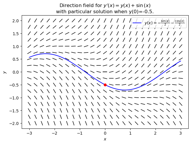
The particular solution to the IVP with initial condition y(0) = -0.5 is

\[\displaystyle y{\left(x \right)} = - \frac{\sin{\left(x \right)}}{2} - \frac{\cos{\left(x \right)}}{2}\]

We can plot the particular solution on top of the direction field that we created by first converting the solution expression to a lambda function that can be evaluated numerically.

yfunc = sympy.lambdify(x, psoln.rhs, modules=["numpy"])
xvals = np.linspace(xmin, xmax, num=100)

plt.figure(fig)  # set the current figure to direction field created above
ax.plot(xvals, yfunc(xvals), color="w", label=f"${sympy.latex(psoln)}$")
ax.set_title(
    f"Direction field for $y'(x)={sympy.latex(ode.rhs)}$"
    "\n"
    f"with particular solution when y({x0})={y0}."
)
ax.plot(0, -1 / 2, "ro")  # plot initial condition point (0,-1/2) in red
ax.legend(loc="upper right")
plt.show()