11: Finite difference methods for boundary value problems.

The shooting method replaces the given BVP with a family of IVPs which it solves numerically until it finds one that closely approximates the desired boundary condition(s). The method of finite differences, on the other hand, imposes the boundary condition(s) exactly and instead approximates the differential equation with “finite differences” which leads to a system of equations that can hopefully be solved by a (numerical) equation solver.

Forward differences and backward differences.

The same germ that lead to Euler’s method gives us the finite difference method, viz., if \(h\) is small and nonzero, then

(34)\[y'(x) \approx \frac{y(x+h) - y(x)}{h}\]

since \(y'(x)\) is the limit of the difference quotient as \(h\to 0\). When \(h>0\), we refer to this approximation as a forward difference, and when \(h<0\) we refer to the approximation as a backward difference. To quantify the error in (34), we appeal (once again) to Taylor’s theorem. Assuming that \(h>0\) and that the exact solution \(y\) has sufficiently many continuous derivatives, Taylor’s theorem

(35)\[y(x+h) = y(x) + y'(x)h + \frac{y''(x)}{2!}h^2 + \frac{y'''(x)}{3!}h^3 + \dots.\]

A bit of algebra then shows us that the forward difference approximation

(36)\[y'(x) = \frac{y(x+h) - y(x)}{h} + O(h)\]

as \(h\to 0\). Furthermore, replacing \(h\) by \(-h\) in (35) gives

(37)\[y(x-h) = y(x) - y'(x)h + \frac{y''(x)}{2!}h^2 - \frac{y'''(x)}{3!}h^3 + \dots.\]

Solving for \(y'(x)\) as before, we see that the backwards difference approximation

(38)\[y'(x) = \frac{y(x) - y(x-h)}{h} + O(h)\]

as \(h\to 0\). Thus, we see that both the forward difference and the backward difference approximations are order 1 accurate.

Central differences and higher-order approximations.

The difference in sign pattern between (35) and (37) has a number of happy consequences. First, subtracting (37) from (35) annihilates all the even order terms. In particular, we have

\[\begin{equation*} y(x+h) - y(x-h) = 2y'(x)h + 2\frac{y'''(x)}{3!}h^3 + \dots. \end{equation*}\]

Solving for \(y'(x)\) here gives the order 2 accurate central difference approximation

(39)\[y'(x) = \frac{y(x+h) - y(x-h)}{2h} + O(h^2)\]

as \(h\to 0\).

But there’s more! Adding (37) and (35) annihilates all the odd order terms so that we have

\[\begin{equation*} y(x+h) + y(x-h) = 2y(x)h + 2\frac{y''(x)}{2!}h^2 + 2\frac{y^{(4)}(x)}{4!}h^4 + \dots. \end{equation*}\]

Solving for \(y''(x)\), we obtain the approximation

(40)\[y''(x) = \frac{y(x+h) - 2y(x) + y(x-h)}{h^2} + O(h^2)\]

as \(h\to 0\). One can play similar games (playing different Taylor series expressions off one another) to obtain even higher order approximations to \(y'(x)\) and \(y''(x)\) as well as approximations approximations for higher-order derivatives as needed.

Finite differences for BVPs.

Suppose that we wish to use the finite difference method to numerically approximate a solution to a BVP of the form

(41)\[\begin{split}y'' &= f(x, y, y'),\\ y(a)&= \alpha,\\ y(b)&= \beta.\end{split}\]

We choose a small, positive step size \(h\) and mesh points \(x_0=a < x_1 < \dots < x_n=b\) so that \(h=x_{i+1}-x_i\) for each \(0\le i < n\). Then equations (39) and (40) may be rewritten as

\[\begin{split}y'(x_i) &= \frac{y(x_{i+1}) -y(x_{i-1})}{2h} + O(h^2),\\ y''(x_i) &= \frac{y(x_{i+1}) - 2y(x_i) + y(x_{i-1})}{h^2} + O(h^2)\end{split}\]

as \(h\to 0\). For \(1\le i\le n-1\), we therefore approximate the ODE of (41) at the \(i\)th mesh point \(x_i\) by the equation

(42)\[\frac{y_{i+1} - 2y_i + y_{i-1}}{h^2} = f\left(x, y_i, \frac{y_{i+1} -y_{i-1}}{2h}\right)\]

while the boundary conditions of (41) are rewritten as \(y_0 = \alpha\) and \(y_n = \beta\). This yields a total of \(n+1\) equations with \(n+1\) unknowns. Therefore, the method of finite differences requires a subroutine to solve the resulting system of equations. Gaussian elimination (or one of its relatives) is usually chosen if the equations (42) are linear in the \(y_i\)’s. Otherwise, some nonlinear method such as Newton’s method (or one of its relatives) is required, but that is a topic for another class.

Advantages and disadvantages.

In practice, achieving acceptable accuracy with a finite difference method requires a very small step-size \(h\) as compared to a shooting method. The smaller the step-size, the greater the number of variables involved in the system of equations. The increase in variables puts pressure on both computing time and memory resources. However, it is important to remember that the shooting method requires the numerical solution to a sequence of IVPs until tolerance is achieved. Though finite difference methods tend to be more memory intensive than shooting methods, there are a number of factors that go into deciding which is more work intensive for a given problem.

Example.

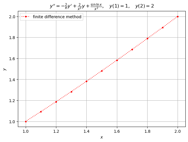
As an example of the centered difference method, we consider the BVP

(43)\[\begin{split}y'' &= -\frac{2}{x}y' + \frac{2}{x^2}y + \frac{\sin(\ln x)}{x^2},\\ y(1) &= 1,\\ y(2) &=2.\end{split}\]

Dividing the interval \([1,2]\) into \(n=10\) equal pieces gives a step-size of \(h = (b - a)/n = 1/10\) and mesh-points

\[\begin{equation*} x_i = a + ih = 1 + i/10\quad (0\le i\le 10). \end{equation*}\]

The central difference approximation (42) yields

\[\begin{equation*} \frac{y_{i+1} -2y_i + y_{i-1}}{h^2} = -\frac{2}{x_i}\left(\frac{y_{i+1} - y_{i-1}}{2h}\right) + \frac{2}{x_i^2}y_i + \frac{\sin(\ln x_i)}{x_i^2} \quad (1\le i\le 9). \end{equation*}\]

Multiplying through by \(-h^2\) and bringing all the \(y_j\)’s over to the left-hand side, we have

\[\begin{equation*} \left(-1-\frac{h}{x_i}\right)y_{i+1} +\left(2+\frac{2}{x_i^2}h^2\right) y_i +\left(-1+\frac{h}{x_i}\right) y_{i-1} = -h^2\frac{\sin(\ln x_i)}{x_i^2} \quad (1\le i\le 9). \end{equation*}\]

The two boundary conditions impose the additional constraints \(y_0 = 1\) and \(y_n = y_{10} = 2\) for a total of \(n+1=11\) equations. We fold the two boundary conditions into the first and last of the finite-difference equations to form a \((n-1)\times (n-1) = 9\times 9\) tridiagonal linear system

\[\begin{equation*} \begin{pmatrix} 2+\frac{2}{x_1^2} & -1-\frac{h}{x_1} & 0 & 0 & \dots & 0\\ -1+\frac{h}{x_2} & 2+\frac{2}{x_2^2} & -1-\frac{h}{x_2} & 0 & \dots & 0\\ 0 & -1+\frac{h}{x_3} & 2+\frac{2}{x_3^2} & -1-\frac{h}{x_3} & \ddots & \vdots\\ \vdots & \ddots & \ddots & \ddots & \ddots & 0\\ \vdots & & \ddots & \ddots & \ddots & -1 -\frac{h}{x_8}\\ 0 & \dots & \dots & 0 & -1+\frac{h}{x_9} & 2+\frac{2}{x_9^2} \end{pmatrix} \begin{bmatrix} y_1\\ y_2\\ y_3 \\ \vdots \\ y_8 \\ y_9 \end{bmatrix} = \begin{bmatrix} -h^2\frac{\sin\ln x_1}{x_1^2} + \left(1-\frac{h}{x_1}\right)y_0\\ -h^2\frac{\sin\ln x_2}{x_2^2}\\ -h^2\frac{\sin\ln x_3}{x_3^2}\\ \vdots\\ -h^2\frac{\sin\ln x_8}{x_8^2}\\ -h^2\frac{\sin\ln x_9}{x_9^2} + \left(1+\frac{h}{x_{9}}\right)y_{10} \end{bmatrix}. \end{equation*}\]

In the code block we below, we construct and solve this system with NumPy tools.

import numpy as np
from matplotlib import pyplot
from tabulate import tabulate

pyplot.style.use("dark_background")

# solve BVP y'' = -(2/x)y' + (2/x^2)y + sin(ln x)/x^2, y(1) = 1, y(2) = 2

a, b = 1, 2
alpha, beta = 1, 2

# construct coefficient matrix A and RHS B
n = 10
h = (b - a) / n
x = np.linspace(a, b, num=n + 1)
sup_diag = np.array([-1 - h / x[i] for i in range(1, n - 1)])
main_diag = np.array([2 + 2 * h**2 / x[i] ** 2 for i in range(1, n)])
sub_diag = np.array([-1 + h / x[i] for i in range(2, n)])
A = np.diag(sup_diag, 1) + np.diag(main_diag) + np.diag(sub_diag, -1)
B = np.array([-(h**2) * np.sin(np.log(x[i])) / x[i] ** 2 for i in range(1, n)])
B[0] += (1 - h / x[1]) * alpha
B[n - 2] += (1 + h / x[n - 1]) * beta

# solve linear system AY = B.
y = np.linalg.solve(A, B)
y = np.insert(y, 0, alpha)
y = np.append(y, beta)

# tabulate the results
data = np.c_[x, y]
hdrs = ["i", "x_i", "y_i"]
print("Finite difference method.")
print(
    tabulate(
        data,
        hdrs,
        tablefmt="mixed_grid",
        floatfmt=["0.0f", "0.1f", "0.8f"],
        showindex=True,
    )
)

# plot solution
fig, ax = pyplot.subplots(layout="constrained")
ax.plot(x, y, "r:.", label=f"finite difference method")
ax.set_title(r"$y'' = -\frac{2}{x}y' + \frac{2}{x^2}y + \frac{\sin\ln x}{x^2},\quad y(1)=1,\quad y(2)=2$")
ax.set_xlabel(r"$x$")
ax.set_ylabel(r"$y$")
ax.legend(loc="upper left")
ax.grid(True)
pyplot.show()

Finite difference method.
┍━━━━━┯━━━━━━━┯━━━━━━━━━━━━┑
│   i │   x_i │        y_i │
┝━━━━━┿━━━━━━━┿━━━━━━━━━━━━┥
│   0 │   1.0 │ 1.00000000 │
├─────┼───────┼────────────┤
│   1 │   1.1 │ 1.09260052 │
├─────┼───────┼────────────┤
│   2 │   1.2 │ 1.18704313 │
├─────┼───────┼────────────┤
│   3 │   1.3 │ 1.28333687 │
├─────┼───────┼────────────┤
│   4 │   1.4 │ 1.38140205 │
├─────┼───────┼────────────┤
│   5 │   1.5 │ 1.48112026 │
├─────┼───────┼────────────┤
│   6 │   1.6 │ 1.58235990 │
├─────┼───────┼────────────┤
│   7 │   1.7 │ 1.68498902 │
├─────┼───────┼────────────┤
│   8 │   1.8 │ 1.78888175 │
├─────┼───────┼────────────┤
│   9 │   1.9 │ 1.89392110 │
├─────┼───────┼────────────┤
│  10 │   2.0 │ 2.00000000 │
┕━━━━━┷━━━━━━━┷━━━━━━━━━━━━┙

The method of central differences applied to the BVP (43) ultimately led to a linear system of equations that could be solved with numerical linear equation solver. This is the case with any linear ODE. Nonlinear ODEs, however, will yield nonlinear systems of equations, and hence will require a nonlinear equation solver.