Physical example: Simple gravity pendulum

\(\newcommand{\dee}{\mathrm{d}}\)

Under certain simplifying assumptions, the motion of a swinging pendulum is described by the ODE

(24)\[\ddot{\theta} + \frac{g}{L}\sin\theta = 0,\]

where \(L\) is the length of the pendulum, \(g\) is the acceleration due to gravity near the Earth’s surface, and \(\theta\) is the angle that the pendulum makes with the vertical axis. To see this, we argue as follows. First, we write

(25)\[\boldsymbol r = \langle x, y\rangle = L\langle \sin\theta, -\cos\theta\rangle\]

for the radial vector describing the position of the bob relative to the anchored end of the pendulum. By the chain rule, the velocity of the bob is

(26)\[\boldsymbol v =\frac{\dee\boldsymbol r}{\dee t} =\frac{\dee\boldsymbol r}{\dee\theta}\frac{\dee\theta}{\dee t} =\dot{\theta}\frac{\dee\boldsymbol r}{\dee\theta}\]

and the acceleration is

(27)\[\boldsymbol a = \frac{\dee\boldsymbol v}{\dee t} =\dot{\theta}\frac{\dee}{\dee t}\left(\frac{\dee\boldsymbol r}{\dee \theta}\right) + \frac{\dee\boldsymbol r}{\dee\theta}\ddot{\theta} =\big(\dot{\theta}\big)^2\frac{\dee^2 \boldsymbol r}{\dee \theta^2} + \ddot{\theta}\frac{\dee\boldsymbol r}{\dee\theta}.\]

Now the total force acting on the bob is

\[\begin{equation*} \boldsymbol F = \boldsymbol F_1 + \boldsymbol F_2 = -mg\hat{\boldsymbol\jmath} + |\boldsymbol F_2|\hat{\frac{\dee^2\boldsymbol r}{\dee\theta^2}}, \end{equation*}\]

where \(m\) is the mass of the bob, \(\boldsymbol F_1 = -mg\hat{\boldsymbol\jmath}\) is the force due to gravity, and \(\boldsymbol F_2 = -|\boldsymbol F_2|\hat{\boldsymbol r} = |\boldsymbol F_2|\hat{\frac{\dee^2\boldsymbol r}{\dee\theta^2}}\) is the force exerted by the rod on the bob. Then Newton’s second law gives the identity \(\boldsymbol F = m\boldsymbol a\). Upon observing that \(\hat{\frac{\dee\boldsymbol r}{\dee\theta}} = \frac{1}{L}\frac{\dee\boldsymbol r}{\dee\theta} = \langle\cos\theta, \sin\theta\rangle\) and \(\hat{\frac{\dee^2\boldsymbol r}{\dee\theta^2}} = \frac{1}{L}\frac{\dee^2\boldsymbol r}{\dee\theta^2} = \langle -\sin\theta, \cos\theta\rangle\) form an orthonormal pair, we see that

\[\begin{equation*} -mg\sin\theta =\boldsymbol F\cdot\hat{\frac{\dee\boldsymbol r}{\dee\theta}} =m\boldsymbol a\cdot\hat{\frac{\dee\boldsymbol r}{\dee\theta}} =mL\ddot{\theta}. \end{equation*}\]

Therefore, dividing through by \(mL\) and adding \(mg\sin\theta\) to each side, we arrive at (24).

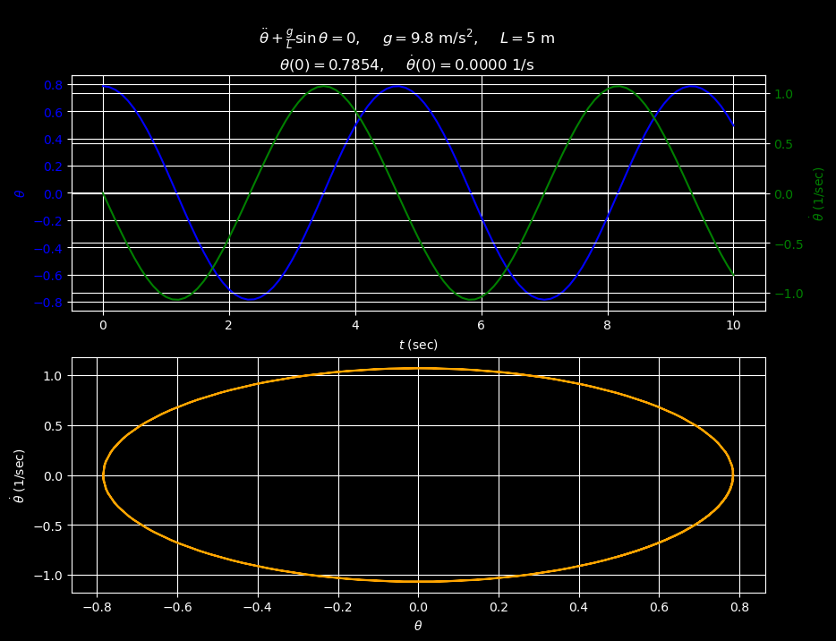
Below we study this model numerically over a 10-second interval assuming that \(g=9.8\) m/s², \(L=5\) m, and imposing the initial conditions \(\theta = \pi/4\) and \(\dot\theta = 0\) s^-1. Our first step is to convert the second-order ODE (24) to a first-order ODE. To that end, we let \(\boldsymbol Y = \langle \theta, \dot\theta\rangle\) and observe that \(\frac{\dee\boldsymbol Y}{\dee t} = \langle \dot\theta, \ddot\theta\rangle\). Then observing that (24) tells us how to compute \(\ddot\theta\) in terms of \(\theta\) (and \(\dot\theta\)), we choose \(\boldsymbol f(t, \boldsymbol Y) = \langle \dot\theta, -\frac{g}{L}\sin\theta\rangle\). Thus, with these definitions, we see that the second-order (scalar) ODE (24) is equivalent to the first-order (vector) ODE

\[\begin{equation*} \frac{\dee\boldsymbol Y}{\dee t} = \boldsymbol f(t, \boldsymbol Y). \end{equation*}\]

# import modules
import numpy
from IPython.display import HTML
from matplotlib import animation, pyplot
from numpy import pi
from numpy.linalg import norm

import math263

# define IVP params
g = 9.8  # acceleration due gravity near surface of Earth (m/s^2)
L = 5  # length of pendulum rod (m)


# rewrite higher-order ODE as first-order system Y' = f(t, Y), where Y = <theta, theta'>
# Y' = <theta', theta''> = <theta', -(g/l)sin(theta)> = f(t, Y)
def f(t, Y):
    theta, theta_dot = Y
    theta_ddot = -(g / L) * numpy.sin(theta)
    return numpy.array([theta_dot, theta_ddot])


# study over a 10-second time-interval 
alpha, beta = 0, 10
# set initial angle and angular velocity
theta0 = pi / 4
theta_dot0 = 0
Y0 = numpy.array([theta0, theta_dot0])

# numerically solve with time-steps of length h = 0.1 secs
h = 0.1
n = int((beta - alpha) / h)
t, Y = math263.rk4(f, alpha, beta, Y0, n)

# extract angles and angular velocities at each time t_i
theta = Y[:, 0]
theta_dot = Y[:, 1]

# make various plots of numerical solution
pyplot.style.use("dark_background")
fig = pyplot.figure()
fig.set_size_inches(10, 7.5)
title = f"""
$\\ddot{{\\theta}} + \\frac{{g}}{{L}}\\sin\\theta = 0,\\quad$ \
$g = {g}\\mathregular{{\\ m/s^2}},\\quad$ \
$L = {L}$ m
$\\theta({alpha}) = {theta0:0.4f},\\quad$ \
$\\dot{{\\theta}}({alpha}) = {theta_dot0:0.4f}\\mathregular{{\\ 1/s}}$
"""
fig.suptitle(title)

# plot \theta (angle) vs t (time)
ax = fig.add_subplot(2, 1, 1)
color = "blue"
ax.plot(t, theta, color=color, label=r"$\theta$")
ax.set_xlabel(r"$t$ (sec)")
ax.set_ylabel(r"$\theta$", color=color)
ax.grid(True)
ax.tick_params(axis="y", labelcolor=color)

# plot \dot\theta (angular velocity) vs t (time)
ax = ax.twinx()
color = "green"
ax.plot(t, theta_dot, color=color, label=r"$\dot\theta$")
ax.set_ylabel(r"$\dot\theta$ (1/sec)", color=color)
ax.grid(True)
ax.tick_params(axis="y", labelcolor=color)

# make phase portrait theta' vs. theta
ax = fig.add_subplot(2, 1, 2)
ax.plot(theta, theta_dot, color="orange")
ax.set_xlabel(r"$\theta$")
ax.set_ylabel(r"$\dot{\theta}$ (1/sec)")
ax.grid(True)

pyplot.show()

Note that equations (25), (26), and (27) tell us how to compute the position, velocity, and acceleration of the bob at any time for which we know both \(\theta\) and \(\dot{\theta}\). We exploit this fact below to produce an animation of the pendulum’s motion in physical space given the numerical values for \(\theta\) and \(\dot{\theta}\) that we computed at \(h = 0.1\)-second intervals.

# compute physical coordinates of the "bob" at each time t_i
x = L * numpy.sin(theta)
y = -L * numpy.cos(theta)

# compute velocity and acceleration vectors
v = theta_dot * L * numpy.array([numpy.cos(theta), numpy.sin(theta)])
v /= max(norm(v, 2, axis=0))
theta_ddot = -(g / L) * numpy.sin(theta)
a = theta_dot**2 * L * numpy.array(
    [-numpy.sin(theta), numpy.cos(theta)]
) + theta_ddot * L * numpy.array([numpy.cos(theta), numpy.sin(theta)])
a /= max(norm(a, 2, axis=0))

# compute edges of window in xy-plane
xmin, xmax = min(x), max(x)
ymin, ymax = min(y), 0
xmin -= 0.5
xmax += 0.5
ymin -= 0.5

# pyplot.style.use("default")
# pyplot.xkcd()
# pyplot.rcParams["font.family"] = ["Comic Sans MS"]
fig, ax = pyplot.subplots()
ax.set_title("Pendulum")

rod = ax.plot([0, x[0]], [0, y[0]], color="blue")[0]  # draw "rod"
bob = ax.scatter(x[0], y[0], color="red", marker="o")  # draw "bob"
vel = pyplot.arrow(x=x[0], y=y[0], dx=v[0, 0], dy=v[1, 0], width=0.05, color="green")
acc = pyplot.arrow(x=x[0], y=y[0], dx=a[0, 0], dy=a[1, 0], width=0.05, color="red")
ax.set_xlim((xmin, xmax))
ax.set_ylim((ymin, ymax))
ax.set_xlabel("$x$ (meters)")
ax.set_ylabel("$y$ (meters)")
pyplot.gca().set_aspect("equal")


def frame_update(frame):
    rod.set_xdata([0, x[frame]])
    rod.set_ydata([0, y[frame]])
    bob.set_offsets([x[frame], y[frame]])
    vel.set_data(x=x[frame], y=y[frame], dx=v[0, frame], dy=v[1, frame])
    acc.set_data(x=x[frame], y=y[frame], dx=a[0, frame], dy=a[1, frame])
    return rod, bob, vel, acc


# we make a new frame for each time-node
# we pause for h * 1000 milliseconds before drawing the next frame
anim = animation.FuncAnimation(
    fig=fig, func=frame_update, frames=len(t), interval=h * 1000
)
pyplot.close()
HTML(anim.to_html5_video())