
8: Higher order initial value problems.#
An \(m\)th order ordinary differential equation in normal form is an equation of the form
To obtain a unique solution, it is typically necessary to specify \(m\) initial conditions, say \(y(x_0) = \alpha_0, y'(x_0) = \alpha_1, \dots, y^{(m-1)}(x_0) = \alpha_{m-1}\). To numerically solve such a problem we introduce \(m\) auxiliary variables (really functions) so as to express the problem as a first order system IVP. Thus, we reduce the problem to one we already know how to solve. More precisely, we let \(u_0=y, u_1=y', \dots, u_{m-1}=y^{(m-1)}\). Then equation (22) is equivalent to the system
In this way, we are able to compute a numerical solution \(y\) to the \(m\)th order IVP along with its lower order derivatives \(y', y'', \dots , y^{(m-1)}\).
Example.#
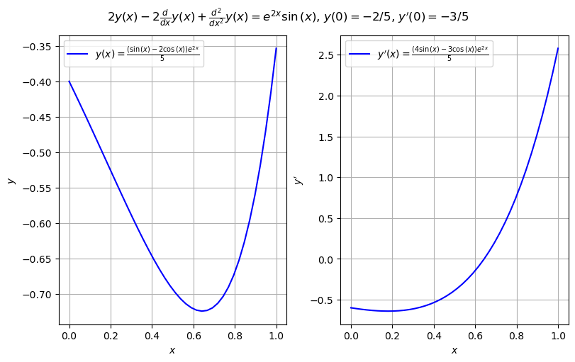
Consider the second-order initial-value problem
import matplotlib.pyplot as plt
import numpy as np
import sympy
from tabulate import tabulate

import math263

#plt.style.use("dark_background")

# solve the IVP symbolically with the sympy library
x = sympy.Symbol("x")
y = sympy.Function("y")
ode = sympy.Eq(
    y(x).diff(x, 2) - 2 * y(x).diff(x) + 2 * y(x), sympy.exp(2 * x) * sympy.sin(x)
)
a, b = 0, 1
alpha = [sympy.Rational(-2, 5), sympy.Rational(-3, 5)]
soln = sympy.dsolve(ode, y(x), ics={y(a): alpha[0], y(x).diff(x).subs(x, a): alpha[1]})
soln = sympy.simplify(soln)

print("The exact symbolic solution to the IVP is")
display(soln)
Dsoln_rhs = sympy.simplify(soln.rhs.diff(x))

# lambdify the symbolic solution
sym_y = sympy.lambdify(x, soln.rhs, modules=["numpy"])
sym_Dy = sympy.lambdify(x, Dsoln_rhs, modules=["numpy"])
xvals = np.linspace(a, b, num=40)

# plot symbolic solution with matplotlib.pyplot
fig, axs = plt.subplots(ncols=2, figsize=(8, 5), layout="constrained")
axs[0].plot(xvals, sym_y(xvals), "b", label=f"${sympy.latex(soln)}$")
axs[1].plot(xvals, sym_Dy(xvals), "b", label=f"$y'(x) = {sympy.latex(Dsoln_rhs)}$")
fig.suptitle(f"${sympy.latex(ode)}$, $y({a}) = {alpha[0]}$, $y'({a}) = {alpha[1]}$")
for i in range(len(axs)):
    axs[i].set_xlabel(r"$x$")
    axs[i].legend(loc="upper left")
    axs[i].grid(True)
axs[0].set_ylabel(r"$y$")
axs[1].set_ylabel(r"$y'$")
plt.show()
The exact symbolic solution to the IVP is
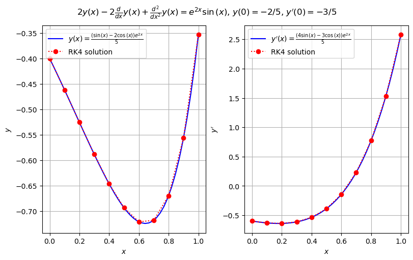
To solve (23) numerically, we introduce the variables \(u_0=y\) \(u_1=y'\), and we rewrite the IVP as
# define IVP parameters
f = lambda x, u: np.array([u[1], 2 * u[1] - 2 * u[0] + np.exp(2 * x) * np.sin(x)])
alpha = [-2 / 5, -3 / 5]

n = 10
(xi, u_rk4) = math263.rk4(f, a, b, alpha, n)

plt.figure(fig)
for i in range(len(axs)):
    axs[i].plot(xi, u_rk4[:, i], "ro:", label="RK4 solution")
    axs[i].legend(loc="upper left")
plt.show()
uvals = np.c_[sym_y(xi), sym_Dy(xi)]
errors = np.abs(uvals - u_rk4)
table = np.c_[xi, u_rk4[:, 0], errors[:, 0], u_rk4[:, 1], errors[:, 1]]
hdrs = ["i", "x_i", "y_i", "|y(x_i) - y_i|", "y_i'", "|y'(x_i) - y_i'|"]
print(tabulate(table, hdrs, tablefmt="mixed_grid",
    floatfmt=["0.0f", "0.2f", "0.5f", "0.5e", "0.5f", "0.5e"], showindex=True))
┍━━━━━┯━━━━━━━┯━━━━━━━━━━┯━━━━━━━━━━━━━━━━━━┯━━━━━━━━━━┯━━━━━━━━━━━━━━━━━━━━┑
│   i │   x_i │      y_i │   |y(x_i) - y_i| │     y_i' │   |y'(x_i) - y_i'| │
┝━━━━━┿━━━━━━━┿━━━━━━━━━━┿━━━━━━━━━━━━━━━━━━┿━━━━━━━━━━┿━━━━━━━━━━━━━━━━━━━━┥
│   0 │  0.00 │ -0.40000 │      0.00000e+00 │ -0.60000 │        1.11022e-16 │
├─────┼───────┼──────────┼──────────────────┼──────────┼────────────────────┤
│   1 │  0.10 │ -0.46173 │      3.71681e-07 │ -0.63163 │        1.91365e-07 │
├─────┼───────┼──────────┼──────────────────┼──────────┼────────────────────┤
│   2 │  0.20 │ -0.52556 │      8.35624e-07 │ -0.64015 │        2.83552e-07 │
├─────┼───────┼──────────┼──────────────────┼──────────┼────────────────────┤
│   3 │  0.30 │ -0.58860 │      1.38949e-06 │ -0.61366 │        1.98967e-07 │
├─────┼───────┼──────────┼──────────────────┼──────────┼────────────────────┤
│   4 │  0.40 │ -0.64661 │      2.02194e-06 │ -0.53658 │        1.67927e-07 │
├─────┼───────┼──────────┼──────────────────┼──────────┼────────────────────┤
│   5 │  0.50 │ -0.69357 │      2.70886e-06 │ -0.38874 │        9.57504e-07 │
├─────┼───────┼──────────┼──────────────────┼──────────┼────────────────────┤
│   6 │  0.60 │ -0.72115 │      3.40851e-06 │ -0.14438 │        2.35303e-06 │
├─────┼───────┼──────────┼──────────────────┼──────────┼────────────────────┤
│   7 │  0.70 │ -0.71815 │      4.05558e-06 │  0.22900 │        4.58994e-06 │
├─────┼───────┼──────────┼──────────────────┼──────────┼────────────────────┤
│   8 │  0.80 │ -0.66971 │      4.55357e-06 │  0.77199 │        7.96642e-06 │
├─────┼───────┼──────────┼──────────────────┼──────────┼────────────────────┤
│   9 │  0.90 │ -0.55644 │      4.76567e-06 │  1.53478 │        1.28552e-05 │
├─────┼───────┼──────────┼──────────────────┼──────────┼────────────────────┤
│  10 │  1.00 │ -0.35340 │      4.50355e-06 │  2.57877 │        1.97163e-05 │
┕━━━━━┷━━━━━━━┷━━━━━━━━━━┷━━━━━━━━━━━━━━━━━━┷━━━━━━━━━━┷━━━━━━━━━━━━━━━━━━━━┙