2: Euler’s method.

Numerical solutions to ODEs.

Suppose that we want to compute a numerical solution to the first-order IVP

(3)\[\begin{split}\begin{align} y'&=f(x,y),\\ y(a) &=y_0 \end{align}\end{split}\]

over the interval \([a,b]\). Choosing some positive integer \(n\), our goal is to compute a sequence of points \((x_i,y_i)\) so that if \(y\) is the true solution, then

\[\begin{equation*} y_i\approx y(x_i) \end{equation*}\]

for \(i = 0,1,\dots, n\). We say that there are \(n\) steps, or equivalently \(n+1\) mesh points or nodes. The distance \(h_i=x_{i+1}-x_i\) is called the \(i\)th step-size, which may be variable. For much of this course, however, we will use equally-spaced meshes with step-size \(h=(b-a)/n\).

Linearization and Euler’s method.

Once the mesh points have been chosen, the most straightforward approach to computing the \(y_i\)’s is known as Euler’s method. It is the method that Katherine Johnson and her team used to compute (mostly by hand) the path that the Apollo astronauts would follow to land on the moon. The basis for Euler’s method is the tangent line approximation from calculus known as linearization. Recall that if \(y\) is differentiable at \(x=x_0\), then

\[\begin{equation*} y(x)\approx y(x_0) + y'(x_0)(x-x_0) \end{equation*}\]

when \(x\) is sufficiently close to \(x_0\). Therefore, if \(y\) is the true solution to the IVP (3) and \(h=x_1-x_0\) is small, then

\[\begin{equation*} y(x_1)\approx y_0 + f(x_0, y_0)h. \end{equation*}\]

Whence choosing \(y_1 = y_0 + hf(x_0, y_0)\), we have \(y_1\approx y(x_1)\) as desired. Continuing in this fashion, Euler’s method is defined by the recurrence

(4)\[y_{i+1} = y_i + f(x_i, y_i)h\]

for \(i\ge 0\).

Python implementation.

The math263 module contains the following Python implementation of Euler’s method.

import numpy as np


def euler(f, a, b, y0, n):
    """
    numerically solves the IVP
        y' = f(x,y), y(a) = y0
    over the interval [a, b] via n steps of Euler's method
    """
    h = (b - a) / n
    x = np.linspace(a, b, num=n + 1)
    y = np.empty((x.size, np.size(y0)))
    y[0] = y0
    for i in range(n):
        y[i + 1] = y[i] + h * f(x[i], y[i])
    return x, y

Example.

We now show how to use Euler’s method to solve the IVP

(5)\[\begin{split}y'&= x^2 - y,\\ y(0)&=3\end{split}\]

over the interval \([0, 2]\).

# load modules
import matplotlib.pyplot as plt
import numpy as np
import sympy
from tabulate import tabulate

import math263

# define IVP parameters
f = lambda x, y: x**2 - y
a, b = 0, 2
y0 = 3

# use the Euler's method from the math263 module to compute numerical solution
n = 10
xi, yi = math263.euler(f, a, b, y0, n)

# tabulate the results
data = np.c_[xi, yi[:, 0]]
hdrs = ["i", "x_i", "y_i"]
print("Euler's method")
print(tabulate(data, hdrs, tablefmt="mixed_grid", floatfmt="0.5f", showindex=True))

Euler's method
┍━━━━━┯━━━━━━━━━┯━━━━━━━━━┑
│   i │     x_i │     y_i │
┝━━━━━┿━━━━━━━━━┿━━━━━━━━━┥
│   0 │ 0.00000 │ 3.00000 │
├─────┼─────────┼─────────┤
│   1 │ 0.20000 │ 2.40000 │
├─────┼─────────┼─────────┤
│   2 │ 0.40000 │ 1.92800 │
├─────┼─────────┼─────────┤
│   3 │ 0.60000 │ 1.57440 │
├─────┼─────────┼─────────┤
│   4 │ 0.80000 │ 1.33152 │
├─────┼─────────┼─────────┤
│   5 │ 1.00000 │ 1.19322 │
├─────┼─────────┼─────────┤
│   6 │ 1.20000 │ 1.15457 │
├─────┼─────────┼─────────┤
│   7 │ 1.40000 │ 1.21166 │
├─────┼─────────┼─────────┤
│   8 │ 1.60000 │ 1.36133 │
├─────┼─────────┼─────────┤
│   9 │ 1.80000 │ 1.60106 │
├─────┼─────────┼─────────┤
│  10 │ 2.00000 │ 1.92885 │
┕━━━━━┷━━━━━━━━━┷━━━━━━━━━┙

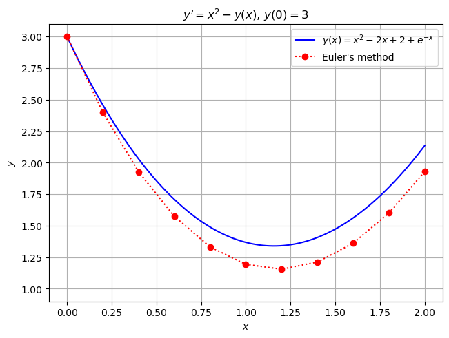
Since the IVP (5) can be solved analytically, we can plot the symbolic and numerical solutions together on the same set of axes.

plt.style.use("dark_background")

# solve the IVP symbolically with the sympy library
x = sympy.Symbol("x")
y = sympy.Function("y")
ode = sympy.Eq(y(x).diff(x), f(x, y(x)))
soln = sympy.dsolve(ode, y(x), ics={y(a): y0})
print("The function")
display(soln)
print("is the exact symbolic solution to the IVP.")
rhs = f(x, y(x))

# convert the symbolic solution to a Python function and plot it with matplotlib.pyplot
sym_y = sympy.lambdify(x, soln.rhs, modules=["numpy"])
xvals = np.linspace(a, b, num=100)
fig, ax = plt.subplots(layout="constrained")
ax.plot(xvals, sym_y(xvals), color="b", label=f"${sympy.latex(soln)}$")
ax.plot(xi, yi[:, 0], "ro:", label="Euler's method")
ax.legend(loc="upper right")
ax.set_title(f"$y' = {sympy.latex(rhs)}$, $y({a})={y0}$")
ax.set_xlabel(r"$x$")
ax.set_ylabel(r"$y$")
ax.grid(True)

The function

\[\displaystyle y{\left(x \right)} = x^{2} - 2 x + 2 + e^{- x}\]

is the exact symbolic solution to the IVP.

Note that although the sequence of errors \(e_i = |y(x_i) - y_i|\) is not necessarily increasing, there is a tendency for the errors made at previous steps to build up at subsequent steps.

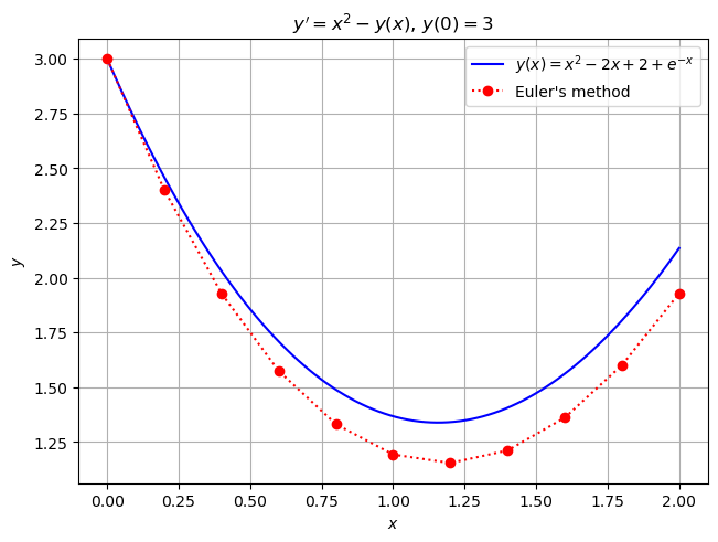
Below we overlay the plot with a direction field plot for the ODE of (5). This helps us to see that every pair of of points \((x_i, y_i)\), \((x_{i+1}, y_{i+1})\) approximates the true solution to the ODE that passes through the point \((x_i, y_i)\), but not necessarily the solution to the given IVP which passes through the initial condition point \((x_0, y_0)\).

# set window boundaries
xmin, xmax = a, b
ymin, ymax = 1, 3

# set step sizes defining the horizontal/vertical distances between mesh points
hx, hy = (b - a) / n, 0.1

# sample x- and y-intervals at appropriate step sizes; explicitly creating array of doubles
xvals = np.arange(xmin, xmax + hx, hx, dtype=np.double)
yvals = np.arange(ymin, ymax + hy, hy, dtype=np.double)

# create rectangle mesh in xy-plane;
X, Y = np.meshgrid(xvals, yvals)
dx = np.ones(X.shape)
# create a dx=1 at each point of the 2D mesh
dy = f(X, Y)
# sample dy =(dy/dx)*dx, where dx=1 at each point of the 2D mesh
# normalize each vector <dx, dy> so that it has "unit" length
[dx, dy] = [dx, dy] / np.sqrt(dx**2 + dy**2)

# plot direction field on top of previous plot
plt.figure(fig)
plt.quiver(
    X, Y, dx, dy, color="w", headlength=0, headwidth=1, pivot="mid", label="_nolegend_"
)
plt.show()