7: Systems of first order ODEs.

An example.

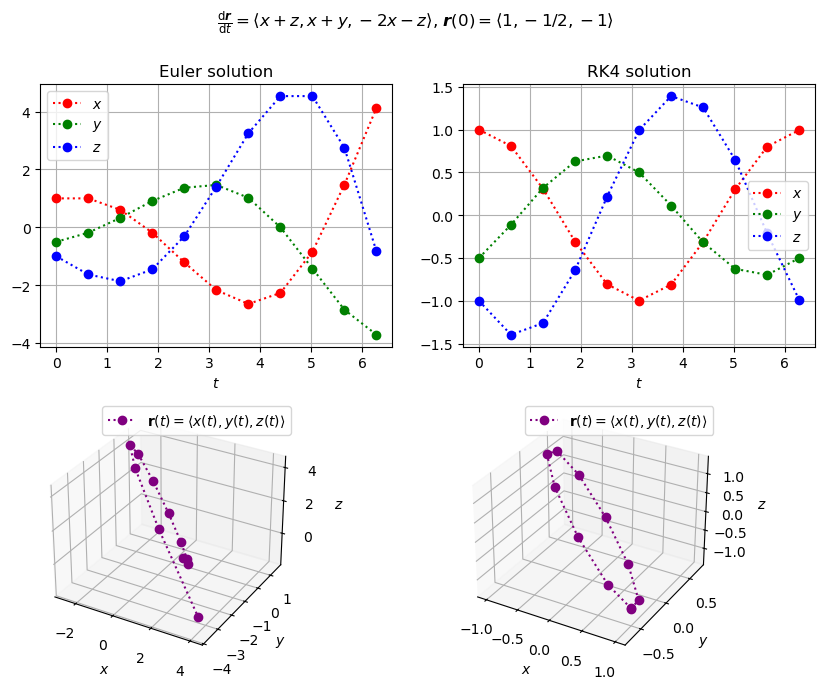
Consider the system of equations

(20)\[\begin{split}\frac{\mathrm{d}x}{\mathrm{d}t} &= x + z,\\ \frac{\mathrm{d}y}{\mathrm{d}t} &= x + y,\\ \frac{\mathrm{d}z}{\mathrm{d}t} &= -2x - z.\end{split}\]

Here it is assumed that \(x\), \(y\), and \(z\) are differentiable functions of \(t\). To specify a unique solution to the system, it is sufficient to impose initial conditions on each function at a given point, say \(x(0) = 1\), \(y(0) = -1/2\), and \(z(0) = -1\), for example.

Since humans are much better at holding onto to one object at time, it is convenient (and conceptually more illuminating) to place collect all 3 scalar-valued functions into a vector-valued function \(\boldsymbol r = \langle x, y, z\rangle\).
Now recall from multivariable calculus that the derivative of a vector-valued function is the vector of derivatives of its scalar component functions. In particular, we have

\[\begin{equation*} \frac{\mathrm{d}\boldsymbol r}{\mathrm{d}t} = \lim_{h\to 0}\frac{\boldsymbol r(t+h) - \boldsymbol r(t)}{h} = \begin{bmatrix} \displaystyle\lim_{h\to 0}\frac{x(t+h) - x(t)}{h}\\ \displaystyle\lim_{h\to 0}\frac{y(t+h) - y(t)}{h}\\ \displaystyle\lim_{h\to 0}\frac{z(t+h) - z(t)}{h} \end{bmatrix} =\begin{bmatrix} \displaystyle\frac{\mathrm{d}x}{\mathrm{d}t}\\ \displaystyle\frac{\mathrm{d}y}{\mathrm{d}t}\\ \displaystyle\frac{\mathrm{d}z}{\mathrm{d}t} \end{bmatrix}. \end{equation*}\]

Note that we write our vectors as columns when displayed, but use the angle-bracket row notation common in multivariable calculus texts as a spacing-saving device for in-line presentation. We also take the liberty of collecting the right-hand sides of (20) into a single vector, writing

\[\begin{equation*} \boldsymbol f(t, \boldsymbol r) = \begin{bmatrix} x + z,\\ x + y,\\ -2x - z \end{bmatrix}. \end{equation*}\]

Furthermore, the initial conditions \(x(0) = 1\), \(y(0) = -1/2\), and \(z(0) = -1\) maybe expressed more compactly as \(\boldsymbol r(0) = \langle 1, -1/2, -1\rangle\).

Now recall that the definition of a vector-valued derivative naturally yields the linear approximation

\[\begin{equation*} \boldsymbol r(t_0+h) \approx \boldsymbol r(t_0) + h\dot{\boldsymbol r}(t_0) \end{equation*}\]

where \(\dot{\boldsymbol r}(t_0) = \frac{\mathrm{d}\boldsymbol r}{\mathrm{d}t}\big|_{t=t_0}\). This of course means that we have the obvious vector-valued extension of Euler’s method, namely

\[\begin{equation*} \boldsymbol r_{i+1} = \boldsymbol r_i + h \boldsymbol f(t_i, \boldsymbol r_i). \end{equation*}\]

Appropriately replacing scalar-valued functions by vector-valued function, we can write down vector-valued versions of all of our numerical methods. For example, the vector-valued extension of RK4 is simply

\[\begin{equation*} \boldsymbol r_{i+1} = \boldsymbol r_i + \frac{h}{6}\big(\boldsymbol k_1 + 2\boldsymbol k_2 + 2\boldsymbol k_3 + \boldsymbol k_4\big), \end{equation*}\]

where

\[\begin{align*} \boldsymbol k_1 &= \boldsymbol f(t_i, \boldsymbol r_i),\\ \boldsymbol k_2 &= \boldsymbol f\big(t_i + h/2, \boldsymbol r_i + h\boldsymbol k_1/2\big),\\ \boldsymbol k_3 &= \boldsymbol f\big(t_i + h/2, \boldsymbol r_i + h\boldsymbol k_2/2\big),\\ \boldsymbol k_4 &= \boldsymbol f(t_i + h, \boldsymbol r_i + h\boldsymbol k_3). \end{align*}\]

Fortunately, many higher-level software packages (e.g., NumPy) have built-in routines and overloaded operators for manipulating vectors as though they were scalars. Since we were careful with our numerical method implementations, this means that our code already works for systems of ODEs. All we need to do is feed the routines appropriately shaped arrays. We demonstrate this below for the system (20).

# load modules
import matplotlib.pyplot as plt
import numpy as np
from numpy import pi
import sympy
from tabulate import tabulate

import math263

# define IVP parameters
f = lambda t, r: np.array([r[0] + r[2], r[0] + r[1], -2 * r[0] - r[2]])
a, b = 0, 2 * pi
r0 = np.array([1, -1 / 2, -1])

# solve with Euler and RK4 methods
n = 10
ti, r_euler = math263.euler(f, a, b, r0, n)
ti, r_rk4 = math263.rk4(f, a, b, r0, n)

# make various plots for each method combined into one figure
plt.style.use("dark_background")
fig = plt.figure()
fig.set_size_inches(10, 7.5)
fig.suptitle(
    r"$\frac{\mathrm{d}\boldsymbol{r}}{\mathrm{d}t} = \langle x+z, x+y, -2x-z\rangle$, "
    r"$\boldsymbol{r}(0) = \langle 1, -1/2, -1\rangle$"
)

# construct x, y, and z vs. t plot for Euler
ax = fig.add_subplot(2, 2, 1)
xi = r_euler[:, 0]
yi = r_euler[:, 1]
zi = r_euler[:, 2]
ax.plot(ti, xi, "ro:", label=r"$x$")
ax.plot(ti, yi, "go:", label=r"$y$")
ax.plot(ti, zi, "bo:", label=r"$z$")
ax.set_title("Euler solution")
ax.set_xlabel(r"$t$")
ax.grid(True)
ax.legend()

# construct parametric plot of r = <x, y, z> for Euler
ax = fig.add_subplot(2, 2, 3, projection="3d")
ax.plot(
    xi,
    yi,
    zi,
    "o:",
    color="purple",
    label=r"$\mathbf{r}(t)=\langle x(t), y(t), z(t)\rangle$",
)
ax.set_xlabel(r"$x$")
ax.set_ylabel(r"$y$")
ax.set_zlabel(r"$z$")
ax.legend()
box = ax.get_position()
box.x0 -= 0.1
ax.set_position(box)
ax.grid(True)

# construct x, y, and z vs. t plot for RK4
ax = fig.add_subplot(2, 2, 2)
xi = r_rk4[:, 0]
yi = r_rk4[:, 1]
zi = r_rk4[:, 2]
ax.plot(ti, xi, "ro:", label=r"$x$")
ax.plot(ti, yi, "go:", label=r"$y$")
ax.plot(ti, zi, "bo:", label=r"$z$")
ax.set_title("RK4 solution")
ax.set_xlabel(r"$t$")
ax.grid(True)
ax.legend()

# construct parametric plot of r = <x, y, z> for RK4
ax = fig.add_subplot(2, 2, 4, projection="3d")
ax.plot(
    xi,
    yi,
    zi,
    "o:",
    color="purple",
    label=r"$\mathbf{r}(t)=\langle x(t), y(t), z(t)\rangle$",
)
ax.set_xlabel(r"$x$")
ax.set_ylabel(r"$y$")
ax.set_zlabel(r"$z$")
ax.legend()
box = ax.get_position()
box.x0 -= 0.1
ax.set_position(box)
ax.grid(True)

plt.show()

Measuring errors with vector norms.

Suppose more generally that \(\boldsymbol r = \langle x_1, \dots, x_m\rangle\), and we seek a solution to the IVP

(21)\[\begin{split}\frac{\mathrm d\boldsymbol r}{\mathrm dt} &= f(t, \boldsymbol r)\\ \boldsymbol r(a) &= \boldsymbol r_0\end{split}\]

over the \(t\)-interval \([a, b]\). To understand errors in higher-dimensional spaces it is helpful to establish the concept of a vector norm.

Definition 3

Suppose that \(\boldsymbol v = \langle v_1,\dots, v_n\rangle\) is a vector in \(n\)-dimensional (real or complex) space. The \(p\)-norm of \(\boldsymbol v\) is the nonnegative real number

\[\begin{equation*} |\boldsymbol v|_p = \begin{cases} \displaystyle\left(\sum_{i=1}^n |v_i|^p\right)^{1/p} & \text{if } p\in (0,\infty),\\ \displaystyle\max_{1\le i\le n}\{|v_i|\} & \text{if } p = \infty. \end{cases} \end{equation*}\]

Vector norms provide a sense of distance in vector spaces that is somewhat akin to a ruler. In particular, we define the \(p\)-distance between two vectors, say \(\boldsymbol v\) and \(\boldsymbol w\), to be the real scalar \(|\boldsymbol v - \boldsymbol w|_p\). Since there are infinitely many choices of \(p\), there are infinitely many choices of “ruler.” Deciding which choice makes the most sense depends on the application. For example, if \(\boldsymbol v\) is a “position vector” in ordinary 3-dimensional space, then the choice \(p=2\) might make sense as it corresponds to the usual euclidean distance. However, there are many situations where the vector \(\boldsymbol v\) is just an “artificial” construct holding a bunch of disparate scalars together for easy manipulation. In such cases, it probably makes more sense to measure distances with the \(\infty\)-norm.

Since (20) can be solved analytically, we solve the system with SymPy. We then compute the absolute error in our RK4 solution at each step \(i\) with both the 2-norm and the \(\infty\)-norm.

# solve the IVP symbolically with the sympy library
t = sympy.Symbol("t")
x = sympy.Function("x")
y = sympy.Function("y")
z = sympy.Function("z")
ode = [
    sympy.Eq(x(t).diff(t), x(t) + z(t)),
    sympy.Eq(y(t).diff(t), x(t) + y(t)),
    sympy.Eq(z(t).diff(t), -2 * x(t) - z(t)),
]
a, b = 0, 2 * pi
soln = sympy.dsolve(
    ode, [x(t), y(t), z(t)], ics={x(a): 1, y(a): sympy.Rational(-1, 2), z(a): -1}
)

# lambdify the symbolic solution
sym_x = sympy.lambdify(t, soln[0].rhs, modules=["numpy"])
sym_y = sympy.lambdify(t, soln[1].rhs, modules=["numpy"])
sym_z = sympy.lambdify(t, soln[2].rhs, modules=["numpy"])
tvals = np.linspace(a, b, num=40)

# tabulate errors for RK4
rvals = np.c_[sym_x(ti), sym_y(ti), sym_z(ti)]
error_vecs = rvals - r_rk4
p = 2
errors_2 = np.linalg.norm(error_vecs, axis=1, ord=p)
errors_inf = np.linalg.norm(error_vecs, axis=1, ord=np.inf)
table = np.c_[ti, errors_2, errors_inf]
print(f"Global {p}-norm and infinity-norm errors for RK4 solution.")
hdrs = ["i", "t_i", "|r(t_i) - r_i|_2", "|r(t_i) - r_i|_inf"]
print(
    tabulate(
        table,
        hdrs,
        tablefmt="mixed_grid",
        floatfmt=["0.0f", "0.5f", "0.5e", "0.5e"],
        showindex=True,
    )
)

Global 2-norm and infinity-norm errors for RK4 solution.
┍━━━━━┯━━━━━━━━━┯━━━━━━━━━━━━━━━━━━━━┯━━━━━━━━━━━━━━━━━━━━━━┑
│   i │     t_i │   |r(t_i) - r_i|_2 │   |r(t_i) - r_i|_inf │
┝━━━━━┿━━━━━━━━━┿━━━━━━━━━━━━━━━━━━━━┿━━━━━━━━━━━━━━━━━━━━━━┥
│   0 │ 0.00000 │        0.00000e+00 │          0.00000e+00 │
├─────┼─────────┼────────────────────┼──────────────────────┤
│   1 │ 0.62832 │        8.54539e-04 │          7.23567e-04 │
├─────┼─────────┼────────────────────┼──────────────────────┤
│   2 │ 1.25664 │        1.58544e-03 │          1.14773e-03 │
├─────┼─────────┼────────────────────┼──────────────────────┤
│   3 │ 1.88496 │        3.36021e-03 │          2.38391e-03 │
├─────┼─────────┼────────────────────┼──────────────────────┤
│   4 │ 2.51327 │        5.28139e-03 │          4.28826e-03 │
├─────┼─────────┼────────────────────┼──────────────────────┤
│   5 │ 3.14159 │        5.95742e-03 │          5.54975e-03 │
├─────┼─────────┼────────────────────┼──────────────────────┤
│   6 │ 3.76991 │        5.12717e-03 │          4.34641e-03 │
├─────┼─────────┼────────────────────┼──────────────────────┤
│   7 │ 4.39823 │        5.53913e-03 │          4.01258e-03 │
├─────┼─────────┼────────────────────┼──────────────────────┤
│   8 │ 5.02655 │        8.94407e-03 │          6.34824e-03 │
├─────┼─────────┼────────────────────┼──────────────────────┤
│   9 │ 5.65487 │        1.18700e-02 │          9.63224e-03 │
├─────┼─────────┼────────────────────┼──────────────────────┤
│  10 │ 6.28319 │        1.19106e-02 │          1.10934e-02 │
┕━━━━━┷━━━━━━━━━┷━━━━━━━━━━━━━━━━━━━━┷━━━━━━━━━━━━━━━━━━━━━━┙