
12: Stiffness.#
A badly-behaved example.#
Consider the initial value problem
over the \(t\)-interval \([0, 1]\). The problem is easy to solve analytically.
import numpy
import sympy
from matplotlib import pyplot
from tabulate import tabulate

import math263

pyplot.style.use("dark_background")

# define IVP parameters
f = lambda t, y: -200 * y + 200 * t + 101
a, b = 0, 1
y0 = 1.01

# solve the IVP symbolically with the sympy library
y = sympy.Function("y")
t = sympy.Symbol("t")
ode = sympy.Eq(y(t).diff(t), f(t, y(t)))
soln = sympy.dsolve(ode, y(t), ics={y(a): y0})
print("The function")
display(soln)
print("is the exact symbolic solution to the IVP.")

# convert the symbolic solution to a Python function and plot it with matplotlib.pyplot
sym_y = sympy.lambdify(t, soln.rhs, modules=["numpy"])
tvals = numpy.linspace(a, b, num=300)
fig, ax = pyplot.subplots(layout="constrained")
ax.plot(tvals, sym_y(tvals), linewidth=2.5, label=f"${sympy.latex(soln)}$")
ax.legend(loc="upper left")
ax.set_title(f"${sympy.latex(ode)}$, $y({a})={y0}$")
ax.set_xlabel(r"$t$")
ax.set_ylabel(r"$y$")
ax.grid(True)
pyplot.show()
The function
is the exact symbolic solution to the IVP.
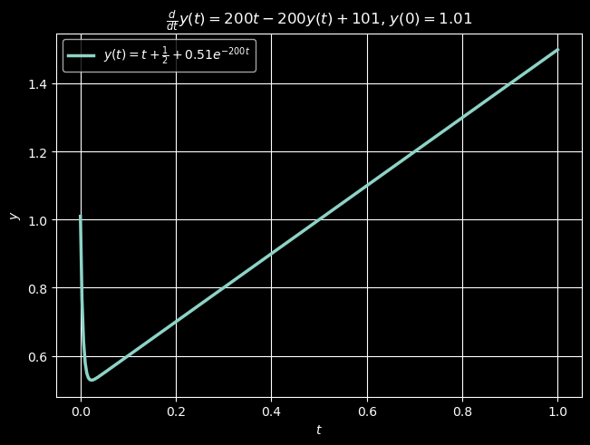
Since the solution \(y\) is (for the most part) slowly varying over the \(t\)-interval \([0, 1]\), it seems that this problem should pose no problem for our numerical methods. However, the Euler method with step-size \(h=0.1\) is awesomely terrible, and RK4 is even worse!
# numerically solve the IVP with forward Euler and RK4
h = 0.1
n = round((b - a) / h)
ti, y_euler = math263.euler(f, a, b, y0, n)
ti, y_rk4 = math263.rk4(f, a, b, y0, n)

# tabulate errors
print("Global errors for Euler's method and RK4.")
table = numpy.c_[ti, abs(sym_y(ti) - y_euler), abs(sym_y(ti) - y_rk4)]
hdrs = ["i", "t_i", "e_{i,Euler} = |y(t_i)-y_i|", "e_{i,RK4} = |y(t_i)-y_i|"]
print(
    tabulate(
        table,
        hdrs,
        tablefmt="mixed_grid",
        floatfmt=["0.0f", "0.2f", "0.5e", "0.5e"],
        numalign="right",
        showindex=True,
    )
)
Global errors for Euler's method and RK4.
┍━━━━━┯━━━━━━━┯━━━━━━━━━━━━━━━━━━━━━━━━━━━━━━┯━━━━━━━━━━━━━━━━━━━━━━━━━━━━┑
│   i │   t_i │   e_{i,Euler} = |y(t_i)-y_i| │   e_{i,RK4} = |y(t_i)-y_i| │
┝━━━━━┿━━━━━━━┿━━━━━━━━━━━━━━━━━━━━━━━━━━━━━━┿━━━━━━━━━━━━━━━━━━━━━━━━━━━━┥
│   0 │  0.00 │                  0.00000e+00 │                0.00000e+00 │
├─────┼───────┼──────────────────────────────┼────────────────────────────┤
│   1 │  0.10 │                  9.69000e+00 │                2.81231e+03 │
├─────┼───────┼──────────────────────────────┼────────────────────────────┤
│   2 │  0.20 │                  1.84110e+02 │                1.55080e+07 │
├─────┼───────┼──────────────────────────────┼────────────────────────────┤
│   3 │  0.30 │                  3.49809e+03 │                8.55164e+10 │
├─────┼───────┼──────────────────────────────┼────────────────────────────┤
│   4 │  0.40 │                  6.64637e+04 │                4.71566e+14 │
├─────┼───────┼──────────────────────────────┼────────────────────────────┤
│   5 │  0.50 │                  1.26281e+06 │                2.60037e+18 │
├─────┼───────┼──────────────────────────────┼────────────────────────────┤
│   6 │  0.60 │                  2.39934e+07 │                1.43393e+22 │
├─────┼───────┼──────────────────────────────┼────────────────────────────┤
│   7 │  0.70 │                  4.55875e+08 │                7.90717e+25 │
├─────┼───────┼──────────────────────────────┼────────────────────────────┤
│   8 │  0.80 │                  8.66162e+09 │                4.36028e+29 │
├─────┼───────┼──────────────────────────────┼────────────────────────────┤
│   9 │  0.90 │                  1.64571e+11 │                2.40440e+33 │
├─────┼───────┼──────────────────────────────┼────────────────────────────┤
│  10 │  1.00 │                  3.12684e+12 │                1.32587e+37 │
┕━━━━━┷━━━━━━━┷━━━━━━━━━━━━━━━━━━━━━━━━━━━━━━┷━━━━━━━━━━━━━━━━━━━━━━━━━━━━┙
Stiffness.#
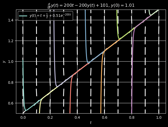
The reason that the above example behaves so poorly is that the desired solution is surrounded by other rapidly decaying transient solutions to the ODE. The fact that these other solutions converge to our desired solution as \(t\to\infty\) should help dampen out the errors in our numerical methods, but the problem here is that the convergence is (relatively) too fast. It is as though the equation is too stable causing the numerical method to become unstable. This condition is known as stiffness. “Physically, stiffness corresponds to a process whose components have highly disparate time scales or a process whose time scale is very short compared to the interval over which it is being studied (Heath. Scientific Computing, 2e., 2002).”
Below we give a plot of the desired solution to the IVP (44) together with several other solutions to the ODE (with different initial value conditions) on top of a direction field. Observe that the slopes of these other solutions are very steep at locations very near the desired solution.
pyplot.figure(fig)
for i in range(1, len(ti)):
    # solve the IVP with initial condition y(t_i) = y_i (from Euler solution)
    solni = sympy.dsolve(ode, y(t), ics={y(ti[i]): y_euler[i]})
    sym_yi = sympy.lambdify(t, solni.rhs, modules=["numpy"])
    tvals = numpy.linspace(ti[i], b, num=300)
    ax.plot(tvals, sym_yi(tvals), linewidth=2.5, label=f"${sympy.latex(solni)}$")

# create direction field for ODE
tmin, tmax = a, b
ymin, ymax = 1 / 2, 3 / 2

# set step sizes defining the horizontal/vertical distances between mesh points
ht, hy = (b - a) / n, 0.1

# sample x- and y-intervals at appropriate step sizes; explicitly creating array of doubles
tvals = numpy.arange(tmin, tmax + ht, ht, dtype=numpy.double)
yvals = numpy.arange(ymin, ymax + hy, hy, dtype=numpy.double)

# create rectangle mesh in xy-plane;
T, Y = numpy.meshgrid(tvals, yvals)
dt = numpy.ones(T.shape)
# create a dx=1 at each point of the 2D mesh
dy = f(T, Y)
# sample dy =(dy/dt)*dt, where dt=1 at each point of the 2D mesh
# normalize each vector <dt, dy> so that it has "unit" length
[dt, dy] = [dt, dy] / numpy.sqrt(dt**2 + dy**2)

# plot direction field on top of previous plot
pyplot.quiver(
    T, Y, dt, dy, color="w", headlength=0, headwidth=1, pivot="mid", label="_nolegend_"
)

pyplot.ylim(ymin, ymax)
pyplot.show()
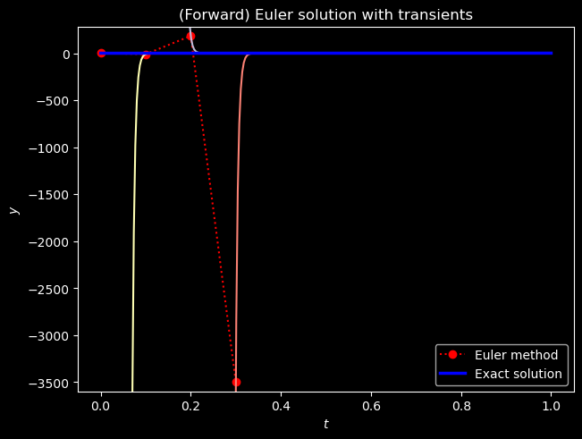
If we plot the first 4 points of the Euler method solution together with each corresponding tangent line, we can see why this situation would tend to “confuse” Euler’s method (or really any explicit method). An explicit method would require a very short step-size \(h\) in order to avoid drastically over-shooting its target.
B = 4
tvals = numpy.linspace(a, b, n)
ymin = min(y_euler[:B])
ymax = max(y_euler[:B])

# create new figure
fig, ax = pyplot.subplots(layout="constrained")
ax.plot(ti[:B], y_euler[:B], "r:o", label="Euler method")
for i in range(B):
    # solve the IVP with initial condition y(t_i) = y_i (from Euler solution)
    solni = sympy.dsolve(ode, y(t), ics={y(ti[i]): y_euler[i]})
    sym_yi = sympy.lambdify(t, solni.rhs, modules=["numpy"])
    tvals = numpy.linspace(a, b, num=300)
    ax.plot(tvals, sym_yi(tvals), label="_nolegend_")
ax.plot(tvals, sym_y(tvals), "b", linewidth=2.5, label="Exact solution")
ax.set_xlabel(r"$t$")
ax.set_ylabel(r"$y$")
ax.set_title("(Forward) Euler solution with transients")
pyplot.ylim(ymin - 100, ymax + 100)
ax.legend()
pyplot.show()
For this reason, stiff differential equations are typically solved using implicit methods, which tend to be much less sensitive to small perturbations in initial conditions. The simplest implicit method is the backward Euler method (BEM), which is defined by the equation (19). By their very nature, implicit methods require an equation solving subroutine. Typically, Newton’s method or some variant is used. For our Python implementation, we decided to use the fsolve routine from the SciPy library.
import numpy as np
import scipy as sp


def bem(f, a, b, y0, n):
    """
    numerically solves the IVP
        y' = f(t, y), y(a)=y0
    over the t-interval [a, b] via n steps of the backward Euler method
    """
    h = (b - a) / n
    t = np.empty(n + 1)
    if np.size(y0) > 1:
        # allocate n + 1 vectors for y
        y = np.empty((t.size, np.size(y0)))
    else:
        # allocate n + 1 scalars for y
        y = np.empty(t.size)
    t[0] = a
    y[0] = y0
    for i in range(n):
        t[i + 1] = t[i] + h
        func = lambda Y: Y - (y[i] + h * f(t[i + 1], Y))
        if np.size(y0) > 1:
            y[i + 1] = sp.optimize.fsolve(func, y[i])
        else:
            y[i + 1] = sp.optimize.fsolve(func, y[i]).item()
    return t, y
Below we observe that the backward Euler method has no trouble with the toy problem that has so stymied both the usual (forward) Euler method and RK4.
# numerically solve the IVP with forward Euler and RK4
h = 0.1
n = round((b - a) / h)
ti, y_bem = math263.bem(f, a, b, y0, n)

# tabulate errors
print("Backward Euler solution.")
table = numpy.c_[ti, y_bem, abs(sym_y(ti) - y_bem)]
hdrs = ["i", "t_i", "y_i", "e_{i,BEM} = |y(t_i)-y_i|"]
print(
    tabulate(
        table,
        hdrs,
        tablefmt="mixed_grid",
        floatfmt=["0.0f", "0.2f", "0.5f", "0.5e"],
        numalign="right",
        showindex=True,
    )
)
Backward Euler solution.
┍━━━━━┯━━━━━━━┯━━━━━━━━━┯━━━━━━━━━━━━━━━━━━━━━━━━━━━━┑
│   i │   t_i │     y_i │   e_{i,BEM} = |y(t_i)-y_i| │
┝━━━━━┿━━━━━━━┿━━━━━━━━━┿━━━━━━━━━━━━━━━━━━━━━━━━━━━━┥
│   0 │  0.00 │ 1.01000 │                0.00000e+00 │
├─────┼───────┼─────────┼────────────────────────────┤
│   1 │  0.10 │ 0.62429 │                2.42857e-02 │
├─────┼───────┼─────────┼────────────────────────────┤
│   2 │  0.20 │ 0.70116 │                1.15646e-03 │
├─────┼───────┼─────────┼────────────────────────────┤
│   3 │  0.30 │ 0.80006 │                5.50696e-05 │
├─────┼───────┼─────────┼────────────────────────────┤
│   4 │  0.40 │ 0.90000 │                2.62236e-06 │
├─────┼───────┼─────────┼────────────────────────────┤
│   5 │  0.50 │ 1.00000 │                1.24874e-07 │
├─────┼───────┼─────────┼────────────────────────────┤
│   6 │  0.60 │ 1.10000 │                5.94640e-09 │
├─────┼───────┼─────────┼────────────────────────────┤
│   7 │  0.70 │ 1.20000 │                2.83162e-10 │
├─────┼───────┼─────────┼────────────────────────────┤
│   8 │  0.80 │ 1.30000 │                1.34841e-11 │
├─────┼───────┼─────────┼────────────────────────────┤
│   9 │  0.90 │ 1.40000 │                6.41931e-13 │
├─────┼───────┼─────────┼────────────────────────────┤
│  10 │  1.00 │ 1.50000 │                3.04201e-14 │
┕━━━━━┷━━━━━━━┷━━━━━━━━━┷━━━━━━━━━━━━━━━━━━━━━━━━━━━━┙
Off-the-shelf solutions.#
The SciPy library implements several IVP solvers. The Radau and BDF solvers implement implicit methods that are suitable for stiff equations while LSODA automatically detects stiffness and switches between an explicit method and an implicit method as needed. See scipy.integrate for more details.