10: Boundary value problems and the shooting method.#
Boundary value problems.#
Side conditions must be imposed in order for a system of ODEs to have a unique a solution. If all the side conditions are imposed at a single point, then the problem is called an initial value problem (IVP). If the side conditions are imposed at more than one point, then we have a boundary value problem (BVP). In typical situations, the conditions are imposed at the endpoints (boundary) of an interval \([a,b]\), which of course explains the name.
Since higher-order equations can be expressed as systems of first order equations, we can restrict attention to problems of the form
over the interval \(a\le x\le b\) together with the condition
where as usual bold symbols denote vectors of the appropriate dimension.
The shooting method.#
The shooting method is a trick for turning this type of problem into a “sequence” of problems that we already know how to solve. The idea is to replace the BVP by an IVP with unknown parameters. In particular, we ignore any conditions imposed on \(\mathbf{y}(b)\) by the boundary condition (31). Then we fix any values of the vector \(\mathbf{y}(a)\) that can be determined from the start; the rest we treat as unknowns. We then “guess” the unknown parameters in \(\mathbf{y}(a)\) and solve the resulting IVP. We then check to see if numerical result satisfies (31) to within desired tolerance.
Example.#
Consider for example the second-order BVP
First we let \(u_0 = y\), \(u_1 = y'\), and we rewrite the BVP (32) as
Then we collect the new variables into vectors \(\mathbf u = \langle u_1, u_2\rangle\), \(\mathbf{f}(x, \mathbf u) = \langle u_1, 4u_0\rangle\), and \(\mathbf{g}(\mathbf{u}(0), \mathbf{u}(1)) = \langle u_0(0), u_0(1)-5\rangle\), and observe that the problem is now expressed in the form of (30) and (31).
For the shooting method, we ignore what the boundary condition \(\mathbf{g} = \mathbf 0\) has to say about \(\mathbf u(1)\). Instead we introduce another unknown parameter \(s\), and we consider the IVP
The goal then is to find a value of \(s = u_1(0) = y'(0)\) so that when we solve the resulting IVP \(u_0(1)\approx 5\), i.e., \(|u_0(1) - 5|\) is within a specified tolerance. Below we make an initial guess of \(s = 1\) and solve the IVP with \(n = 10\) steps of RK4.
import numpy
from matplotlib import pyplot
from tabulate import tabulate
from scipy.optimize import fsolve

import math263

#pyplot.style.use("dark_background")

# set up IVP parameters
f = lambda x, u: numpy.array([u[1], 4 * u[0]])
a, b = 0, 1
bcond = 0, 5
# boundary conditions on y = u_0
u0 = lambda s: numpy.array([0, s])
# set u_1(0) = s unknown

# numerically solve the IVP with n = 10 steps of RK4
n = 10
s = 1
xi, ui = math263.rk4(f, a, b, u0(s), n)

print(f"With s = {s}, we have y_{n} = u_{0, n} = {ui[-1, 0]:0.6g}.")

fig, ax = pyplot.subplots(layout="constrained")
ax.plot([a, b], bcond, "go")
ax.plot(xi, ui[:, 0], ":.", label=f"RK4 $s$ = {s}")
ax.set_title(r"$y'' = 4y, y(0)=0, y(1)=5$")
ax.set_xlabel(r"$x$")
ax.set_ylabel(r"$y$")
ax.grid(True)
ax.legend(loc="upper left")
pyplot.show()
With s = 1, we have y_10 = u_(0, 10) = 1.81339.
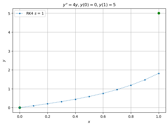
The guess \(s=1\) produces an approximate value for \(y(1) = u_0(1)\) that is too low. This suggests that we should try a steeper guess for \(s = u_1(0) = y'(0)\). Below we try again with \(s=2\).
# numerically solve the IVP with n = 10 steps of RK4
n = 10
s = 2
xi, ui = math263.rk4(f, a, b, u0(s), n)

print(f"With s = {s}, we have y_{n} = u_{0, n} = {ui[-1, 0]:0.6g}.")

pyplot.figure(fig)
ax.plot(xi, ui[:, 0], ":.", label=f"RK4 $s$ = {s}")
ax.set_xlabel(r"$x$")
ax.set_ylabel(r"$y$")
ax.legend(loc="upper left")
pyplot.show()
With s = 2, we have y_10 = u_(0, 10) = 3.62677.
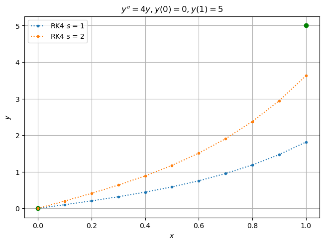
Again we are too low, and so we try \(s=3\).
# numerically solve the IVP with n = 10 steps of RK4
n = 10
s = 3
xi, ui = math263.rk4(f, a, b, u0(s), n)

print(f"With s = {s}, we have y_{n} = u_{0, n} = {ui[-1, 0]:0.6g}.")

pyplot.figure(fig)
ax.plot(xi, ui[:, 0], ":.", label=f"RK4 $s$ = {s}")
ax.set_xlabel(r"$x$")
ax.set_ylabel(r"$y$")
ax.legend(loc="upper left")
pyplot.show()
With s = 3, we have y_10 = u_(0, 10) = 5.44016.
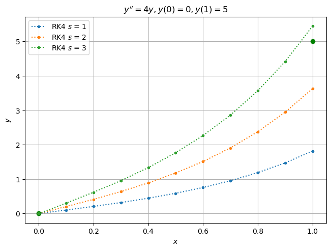
This time we are too high, and that is fortunate for now we have “bracketed” \(s\). In particular, we “know” (assuming that the solution varies continuously with \(s\)) that \(s\in (2,3)\). We can therefore bisect the interval and guess \(s=(2+3)/2=5/2\). If that guess is too low, we know that \(s\in(5/2, 3)\). If it is too high, we know that \(s\in (2, 5/2)\). We can then keep bisecting until our computed value \(u_{0,n} = y_n\) is within some desired tolerance of our target \(y(1)=5\). In practice, it is a good idea to set a maximum number of iterations in case the convergence is rather slow and the work cost is too high.
# tabulate the results for last iteration
data = numpy.c_[xi, ui[:, 0]]
hdrs = ["i", "x_i", "y_i"]
print(
    f"Shooting method (s = {s})\nBoundary error: |y({b})-y_{n}| = {abs(ui[-1,0]-bcond[1]):0.5g}"
)
print(tabulate(data, hdrs, tablefmt="mixed_grid", floatfmt="0.5f", showindex=True))
Shooting method (s = 3)
Boundary error: |y(1)-y_10| = 0.44016
┍━━━━━┯━━━━━━━━━┯━━━━━━━━━┑
│   i │     x_i │     y_i │
┝━━━━━┿━━━━━━━━━┿━━━━━━━━━┥
│   0 │ 0.00000 │ 0.00000 │
├─────┼─────────┼─────────┤
│   1 │ 0.10000 │ 0.30200 │
├─────┼─────────┼─────────┤
│   2 │ 0.20000 │ 0.61612 │
├─────┼─────────┼─────────┤
│   3 │ 0.30000 │ 0.95497 │
├─────┼─────────┼─────────┤
│   4 │ 0.40000 │ 1.33214 │
├─────┼─────────┼─────────┤
│   5 │ 0.50000 │ 1.76277 │
├─────┼─────────┼─────────┤
│   6 │ 0.60000 │ 2.26415 │
├─────┼─────────┼─────────┤
│   7 │ 0.70000 │ 2.85640 │
├─────┼─────────┼─────────┤
│   8 │ 0.80000 │ 3.56328 │
├─────┼─────────┼─────────┤
│   9 │ 0.90000 │ 4.41317 │
├─────┼─────────┼─────────┤
│  10 │ 1.00000 │ 5.44016 │
┕━━━━━┷━━━━━━━━━┷━━━━━━━━━┙
As an alternative to the method of bisection, we may write a function that, given a choice of \(s = u'(0)\), will “shoot” our IVP solver and then return its approximation to \(u(1)-5\), which we want to be zero. We can then feed this function to any numerical equation solver as below and compute \(s\) to our desired tolerance.
# define "shooting" function
def shoot(s):
s = s[0]
soln = math263.rk4(f, a, b, u0(s), n)
u = soln[1]
return u[-1, 0] - bcond[1]
# using SciPy's fsolve to automate search for s
s0 = 3
s = fsolve(shoot, [s0], xtol=1e-5)
s = s[0]
# recompute numerical solution with value returned by eqn solver
xi, ui = math263.rk4(f, a, b, u0(s), n)
# report results
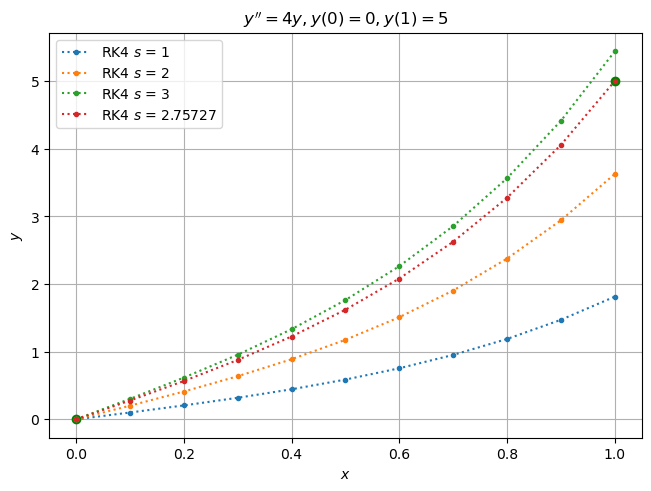
print(f"With s = {s:0.5f}, we have y_{n} = u_{0, n} = {ui[-1, 0]:0.6g}.")
pyplot.figure(fig)
ax.plot(xi, ui[:, 0], ":.", label=f"RK4 $s$ = {s:0.5f}")
ax.set_xlabel(r"$x$")
ax.set_ylabel(r"$y$")
ax.legend(loc="upper left")
pyplot.show()
With s = 2.75727, we have y_10 = u_(0, 10) = 5.