4: Runge–Kutta methods.

The Runge–Kutta methods are a family of numerical methods which generalize both Euler’s method (4) and Heun’s modified Euler method (8). Indeed, the Runge-Kutta method of order \(1\) is Euler’s method, while Heun’s modified Euler method is an example of a second order Runge–Kutta method. The essence of the Runge-Kutta methods is to approximate the true solution using additional terms of the Taylor series without actually computing the higher order derivatives.

Rethinking Heun’s modified Euler method.

Previously, we derived Heun’s modified Euler method based on numerical integration via the trapezoidal rule. We now take a different viewpoint that leads to the development of a whole family of second order methods.

Suppose as usual that we are given an IVP of the form

\[\begin{split}y' &= f(x,y),\\ y(x_0) &= y_0,\end{split}\]

and our goal is to approximate \(y(x_1)\), where \(x_1 = x_0+h\). The Taylor series approach previously developed tells us that to first order we can do no better than Euler’s method, viz,

\[y(x_1) \approx y(x_0) + y'(x_0)(x_1-x_0) = y_0 + f(x_0,y_0)h.\]

The Taylor series approach also makes it clear that to obtain a second order approximation, we require an estimate for \(y''(x_0)\). Now numerical methods are mostly just ways of faking limits. Indeed, if \(\alpha\) is constant with repect to \(h\), then under reasonable assumptions on \(f\) and the solution \(y\), we have

\[\begin{split}y''(x_0) &= \lim_{h\to 0}\frac{y'(x_0+h) - y'(x_0)}{h}\\ &=\frac{y'(x_0+\alpha h) - y'(x_0)}{\alpha h} + O(h)\\ &=\frac{k_1-k_2}{\alpha h} + O(h)\end{split}\]

as \(h\to 0\), where \(k_1 = f(x_0, y_0)\) and \(k_2 = f(x_0+\alpha h, y_0 + \alpha hk_1)\). This estimate then yields second order approximation for \(y(x_1)\), namely,

\[\begin{split}y(x_1) &= y(x_0) + y'(x_0)h +\frac{y''(x_0)}{2}h^2 + O(h^3)\\ &= y_0 + k_1h + \frac{k_2-k_1}{2\alpha h}h^2 + O(h^3)\end{split}\]

as \(h\to 0\). The generic Runge–Kutta method of order 2 is therefore defined by the recurrence

(9)\[y_{i+1} = y_i + h\left(w_1k_1 + w_2k_2\right),\]

where

\[\begin{split}k_1 &= f(x_i, y_i),\\ k_2 &= f(x_i + \alpha h, y_i + h\alpha k_1),\\ w_1 &= 1-\frac{1}{2\alpha},\\ w_2 &= \frac{1}{2\alpha},\end{split}\]

and \(\alpha\) is any positive constant. We mention the three most common choices here. Setting \(\alpha=1\) yields Heun’s (modified Euler) method which we have already met. Ralston’s order 2 method, which also occasionally goes by the name “Heun’s method,” arises by setting \(\alpha=2/3\). Finally, the midpoint method (or corrected Euler method) is defined by the choice \(\alpha=1/2\).

Higher-order methods.

It is natural to speculate that higher-order methods could be obtained by taking a weighted average of additional (approximate) slopes “sampled” from the subinterval \([x_i, x_{i+1}]\). An \(s\)-stage Runge–Kutta method is the result of an average of \(s\) such samples. The general form of an \(s\)-stage method is

(10)\[y_{i+1} = y_i + h\sum_{j=1}^s b_jk_j,\]

where

\[\begin{split}k_1 &= f(x_i, y_i),\\ k_2 &= f(x_i + c_2h, y_i + ha_{2,1}k_1),\\ &\vdots\\ k_s &= f\big(x_i + c_sh, y_i + h(a_{s,1}k_1 + \dots + a_{s,s-1}k_s)\big).\end{split}\]

Of course care must be taken when choosing the coefficients so that the method is consistent with the Taylor series of the true solution.

Perhaps the most popular Runge–Kutta method is the classical fourth order Runge–Kutta method (RK4), which is defined by the recurrence

(11)\[\begin{equation} y_{i+1} = y_i + \frac{h}{6}\big(k_1 + 2k_2 + 2k_3 + k_4\big), \end{equation}\]

where

(12)\[\begin{align} k_1 &= f(x_i, y_i),\\ k_2 &= f\big(x_i + h/2, y_i + hk_1/2\big),\\ k_3 &= f\big(x_i + h/2, y_i + hk_2/2\big),\\ k_4 &= f(x_i + h, y_i + hk_3). \end{align}\]

As the name would seem to imply, RK4 is an order \(4\) numerical method.

A Python implemenation of RK4.

The following Python implementation of RK4 is included in the math263 module.

import numpy as np


def rk4(f, a, b, y0, n):
    """
    numerically solves the IVP
        y' = f(x,y), y(a)=y0
    over the interval [a, b] via n steps of the 4th order (classical) Runge–Kutta method
    """
    h = (b - a) / n
    x = np.linspace(a, b, num=n + 1)
    y = np.empty((x.size, np.size(y0)))
    y[0] = y0
    for i in range(n):
        k1 = f(x[i], y[i])
        k2 = f(x[i] + h / 2, y[i] + h * k1 / 2)
        k3 = f(x[i] + h / 2, y[i] + h * k2 / 2)
        k4 = f(x[i] + h, y[i] + h * k3)
        y[i + 1] = y[i] + h * (k1 + 2 * (k2 + k3) + k4) / 6
    return x, y

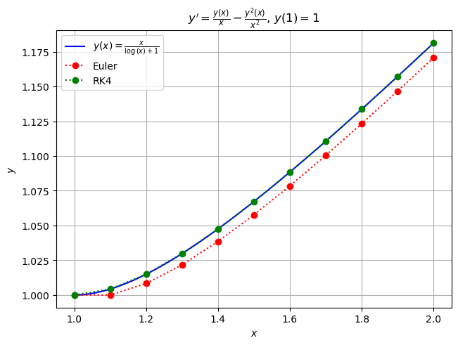
Example.

Below we compare Euler’s method with the classical Runge–Kutta method of order 4 (RK4) for the IVP

(13)\[\begin{align} y'&=(y/x)-(y/x)^2,\\ y(1)&=1. \end{align}\]

import matplotlib.pyplot as plt
import numpy as np
import sympy
from tabulate import tabulate

import math263

plt.style.use("dark_background")

# define IVP parameters
f = lambda x, y: (y / x) - (y / x) ** 2
a, b = 1, 2
y0 = 1

# solve the IVP symbolically with the sympy library
x = sympy.Symbol("x")
y = sympy.Function("y")
ode = sympy.Eq(y(x).diff(x), f(x, y(x)))
soln = sympy.dsolve(ode, y(x), ics={y(a): y0})
print("The exact symbolic solution to the IVP")
display(ode)
print(f"with initial condition y({a}) = {y0} is")
display(soln)

# convert the symbolic solution to a Python function and plot it with matplotlib.pyplot
sym_y = sympy.lambdify(x, soln.rhs, modules=["numpy"])
xvals = np.linspace(a, b, num=100)
fig, ax = plt.subplots(layout="constrained")
ax.plot(xvals, sym_y(xvals), color="b", label=f"${sympy.latex(soln)}$")
ax.set_title(f"$y' = {sympy.latex(f(x,y(x)))}$, $y({a})={y0}$")
ax.set_xlabel(r"$x$")
ax.set_ylabel(r"$y$")
ax.legend([f"${sympy.latex(soln)}$"], loc="upper right")
plt.grid(True)

# numerically solve the IVP with n=10 steps of forward Euler and n=10 steps of RK4
n = 10
xi, y_euler = math263.euler(f, a, b, y0, n)
xi, y_rk4 = math263.rk4(f, a, b, y0, n)

# plot numerical solutions on top of true solution
ax.plot(xi, y_euler[:, 0], "ro:", label="Euler")
ax.plot(xi, y_rk4[:, 0], "go:", label="RK4")
ax.legend(loc="upper left")
plt.show()

# tabulate the results
print("Global errors for Euler's method and RK4.")
table = np.c_[xi, abs(sym_y(xi) - y_euler[:, 0]), abs(sym_y(xi) - y_rk4[:, 0])]
hdrs = ["i", "x_i", "e_{i,Euler} = |y(x_i)-y_i|", "e_{i,RK4} = |y(x_i)-y_i|"]
print(
    tabulate(
        table,
        hdrs,
        tablefmt="mixed_grid",
        floatfmt=["0.0f", "0.1f", "0.5e", "0.5e"],
        showindex=True,
    )
)

The exact symbolic solution to the IVP

\[\displaystyle \frac{d}{d x} y{\left(x \right)} = \frac{y{\left(x \right)}}{x} - \frac{y^{2}{\left(x \right)}}{x^{2}}\]

with initial condition y(1) = 1 is

\[\displaystyle y{\left(x \right)} = \frac{x}{\log{\left(x \right)} + 1}\]

Global errors for Euler's method and RK4.
┍━━━━━┯━━━━━━━┯━━━━━━━━━━━━━━━━━━━━━━━━━━━━━━┯━━━━━━━━━━━━━━━━━━━━━━━━━━━━┑
│   i │   x_i │   e_{i,Euler} = |y(x_i)-y_i| │   e_{i,RK4} = |y(x_i)-y_i| │
┝━━━━━┿━━━━━━━┿━━━━━━━━━━━━━━━━━━━━━━━━━━━━━━┿━━━━━━━━━━━━━━━━━━━━━━━━━━━━┥
│   0 │   1.0 │                  0.00000e+00 │                0.00000e+00 │
├─────┼───────┼──────────────────────────────┼────────────────────────────┤
│   1 │   1.1 │                  4.28173e-03 │                2.24147e-07 │
├─────┼───────┼──────────────────────────────┼────────────────────────────┤
│   2 │   1.2 │                  6.68785e-03 │                3.10759e-07 │
├─────┼───────┼──────────────────────────────┼────────────────────────────┤
│   3 │   1.3 │                  8.12422e-03 │                3.46369e-07 │
├─────┼───────┼──────────────────────────────┼────────────────────────────┤
│   4 │   1.4 │                  9.01919e-03 │                3.60986e-07 │
├─────┼───────┼──────────────────────────────┼────────────────────────────┤
│   5 │   1.5 │                  9.59416e-03 │                3.66382e-07 │
├─────┼───────┼──────────────────────────────┼────────────────────────────┤
│   6 │   1.6 │                  9.97159e-03 │                3.67611e-07 │
├─────┼───────┼──────────────────────────────┼────────────────────────────┤
│   7 │   1.7 │                  1.02229e-02 │                3.66990e-07 │
├─────┼───────┼──────────────────────────────┼────────────────────────────┤
│   8 │   1.8 │                  1.03915e-02 │                3.65627e-07 │
├─────┼───────┼──────────────────────────────┼────────────────────────────┤
│   9 │   1.9 │                  1.05048e-02 │                3.64068e-07 │
├─────┼───────┼──────────────────────────────┼────────────────────────────┤
│  10 │   2.0 │                  1.05806e-02 │                3.62576e-07 │
┕━━━━━┷━━━━━━━┷━━━━━━━━━━━━━━━━━━━━━━━━━━━━━━┷━━━━━━━━━━━━━━━━━━━━━━━━━━━━┙